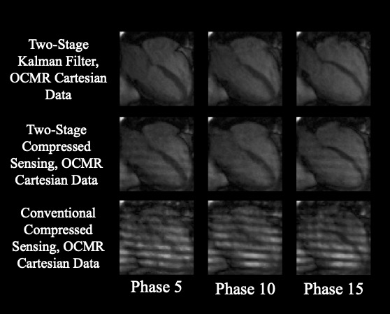
I optimized a signal model for real-time CINE MRI, originally conceived by Aaron Curtis, by developing mathematical techniques that improved computation time by a factor of 1000. These optimizations made the model feasible for clinical application and enabled its integration into compressed sensing algorithms.

CINE MRI is a critical imaging technique used to capture the dynamic motion of the heart in real-time, offering detailed visualizations of cardiac function across multiple phases of the cardiac cycle. This method is particularly valuable for diagnosing and assessing various heart conditions, including heart failure, which is prevalent worldwide. With heart failure affecting millions of people, accurate and timely imaging is essential for effective treatment and management. Real-time CINE MRI enables clinicians to observe the heart’s motion in detail, providing insights that are vital for diagnosing cardiac diseases and guiding interventions.
Traditional compressed sensing methods have been employed to accelerate MRI acquisition, particularly in CINE MRI, where capturing the fast-moving heart requires rapid data collection. These methods rely on the assumption that MR images are sparse in some transform domain, such as the wavelet domain. By undersampling the k-space data and applying sparsity constraints during reconstruction, compressed sensing allows for faster imaging while still maintaining acceptable image quality. However, these techniques often struggle with balancing acceleration and image quality, especially in low-SNR environments or when trying to achieve extremely high acceleration rates.
To enhance real-time CINE MRI reconstruction, we introduce a novel approach that incorporates a linear signal model into the reconstruction process. By learning a linear transform that describes the transition between successive heart phases, we can significantly reduce computation time and improve the accuracy of the reconstructed images. This approach builds on the foundation of traditional compressed sensing but adds an additional layer of model-based optimization, making it particularly well-suited for real-time applications.
My colleague, Aaron Curtis, initially conceived the idea of using a linear model for heart motion, applying it to a Maximum Likelihood Estimation (MLE) filter and later a Kalman filter. My contribution involved developing mathematical derivations that not only reduced computation time but also facilitated clinical application, with potential integration into compressed sensing algorithms.
The algorithm is specifically designed for CINE MRI, focusing on the reconstruction of a single heartbeat across multiple phases. The primary goal is to determine a linear transform that accurately describes the transition from one heart phase to the next.
We start with a single heartbeat CINE reconstruction with \( T \) phases. The primary objective is to determine a linear transform that describes the transition from one phase to the next. Generally, there are infinitely many possible linear transforms that can achieve this. To illustrate, consider points \( x \) and \( y \) in a two-dimensional space and try to determine a matrix \( \mathrm{A} \) such that \( y = \mathrm{A}x \). There are infinite possibilities for \( \mathrm{A} \), and this is analogous to the situation we face.
In our case, we seek an affine transform in the following format:
\[ x_{t+1} = \mathrm{F}x_t \]Here, \( x_t \) is a vectorized image of the heart at phase \( t \), and \( \mathrm{F} \) is the linear transform we need to determine. One approach to determine \( \mathrm{F} \) is to use a Linear Minimum Mean Squared Error (LMMSE) estimator. The equations to determine \( \mathrm{F} \) are as follows:
\[ \mathrm{F} = \mathrm{C_1}\mathrm{C_0}^{-1} \] \[ \mathrm{C_l} = \mathrm{X_l}\mathrm{X^H} \]In this context, \( \mathrm{X} \) is a matrix where the \( t^{th} \) column is set to \( x_t \), and \( \mathrm{X_l} \) is \( \mathrm{X} \) circularly shifted to the left \( l \) times. Unfortunately, \( \mathrm{C_0} \) is not invertible, and even if it were, the matrix would be too large for efficient computation. To address this, we operate within the subspace spanned by \( x_t \), which allows us to rewrite the above equations as:
\[ e_{t+1} = \mathrm{G}e_t \] \[ \mathrm{G} = \mathrm{D_1}\mathrm{D_0}^{-1} \] \[ \mathrm{D_l} = \mathrm{I_l}\mathrm{I^H} \]Here, \( e_t \) represents the standard basis vectors, and \( \mathrm{I_l} \) is the identity matrix circularly shifted to the left \( l \) times. This simplification leads to:
\[ \mathrm{G} = \mathrm{I_1} \]We can now express the transition as follows:
\[ x_{t+1} = \mathrm{XI_1}\left(X^H X\right)^{-1}\mathrm{X}x_t \]This equation shows that the linear transform we were seeking is \( \mathrm{XI_1}\left(X^H X\right)^{-1}\mathrm{X} \). Below shows the result of this signal model applied to a Kalman filtering algorithm and a compressed sensing algorithm. A standard compressed sensing implementation without a signal model is also shown for comparison.
